Mechanical System Modeling

The equations of motion involving a rotary flexible link, involves modeling the rotational base and the flexible link as rigid bodies. As a simplification to the partial differential equation describing the motion of a flexible link, a lumped single degree of freedom approximation is used. We first start the derivation of the dynamic model by computing various rotational moment of inertia terms. The rotational inertia for a flexible link and a light source attachment is given respectively by

where m_link is the total mass of the flexible link, m_light is the mass of the light source compartment, and L is the total flexible link length. Combining the moment of inertia’s for both the link and the light source gives

For a single degree of freedom system, the natural frequency is related with torsional stiffness and rotational inertia in the following manner

where w _n is found experimentally and K_stiff is an equivalent torsion spring constant as delineated through the following figure

In addition, any frictional damping effects between the rotary base and the flexible link are assumed negligible. Next, we derive the generalized dynamic equation for the tip and base dynamics using Lagrange’s energy equations in terms of a set of generalized variables a and q, where a is the angle of tip deflection and q is the base rotation given in the following

where T is the total kinetic energy of the system, P is the total potential energy of the system, and Q_i is the i^th generalized force within the i^th degree of freedom. Kinetic energy of the the base and the flexible link are given respectively as

The total kinetic energy of the mechanical system is computed as the sum of (7) and (8)

Potential energy of the system provided by the torsional spring given as

Applying equation (9) and (10) into (5) and (6) results in the following dynamic equations

Next we compute the amount of virtual work, W, applied into the system. The amount of virtual work is given to be

where t is the torque applied to the rotational base. Rewriting equation (13) into a general form of virtual work given as

We obtain the virtual forces applied onto the generalized coordinatesQq and Qa , respectively to be

After decoupling the acceleration terms of (11) and (12), the dynamic equations for the mechanical subsystem are

Next, rewriting equations (17) and (18) into a state space form gives

Electrical System Modeling

Since the control input into the mechanical model of equation (19) is a torque t , an electrical dynamic equation relating voltage to torque is needed. First, the torque applied to the rotational base, on the right hand side of equation (19), is converted to the torque applied to the gear train by the DC servomotor by means of a gear ratio K_g given as

where t _m is the torque applied by the servomotor. Next, the circuitry within the DC motor system consists of a resistor, an inductor, an external voltage source, and a back emf placed in a series circuit. The following figure describes the circuit as previously described

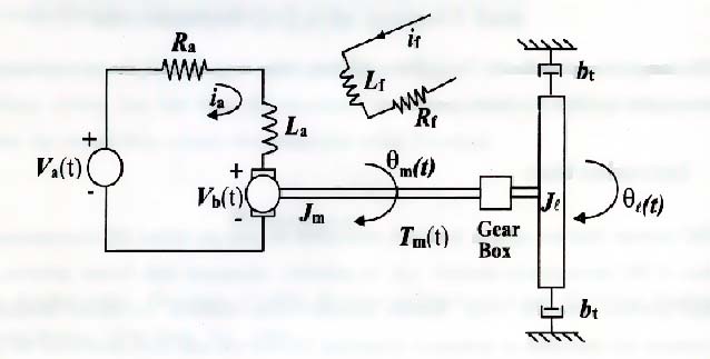
Applying Kirchoff’s voltage law to the above figure, produces

where I is the current in the circuit, R is the resistor, L is the inductor, V_b is the back emf, and V_PC is the voltage supplied by the data acquisition board. The DC servomotor is an electromechanical device that relates torque to current through a proportionality gain K_T given in the following equation

In addition, the back emf is a voltage applied by the motor shaft to the circuit, which is directly proportional to the angular velocity of the motor

where K_b is the back emf constant and w _m is the angular velocity of the motor. Relating the motor angular velocity with the base angular velocity gives

Substituting equations (22) and (24) into (21) gives

Since the effect of the inductance in the circuit is relatively small in comparison with other circuit components, the derivative term of torque can be neglected eliminated to give the following approximate proportionality equation between voltage to torque and angular velocity

The torque applied by the motor is solved for in equation (26) to be

As a result, the state space model of (19) can be rewritten to utilize an electrical control voltage in (20) and (27) to give

Next, a transformation between relative angular position and relative displacement about a neutral axis is used within the state space model of (28). The relative angular position, velocity with respect to the rotating base is proportional to the relative displacement, velocity of the flexible link tip (i.e. sin(a)»a)

The following figure shows the relationship of these three parameters.

Substituting the above equations of (29) and (30) into the state space dynamics of (28) gives the following state space equation

Control Objective

The objective for the rotary flexible link dynamic system is to achieve an asymptotically stable system response for flexible link. A Linear Quadratic Regulator (LQR) based controller achieves asymptotic stable response for a controllable state space model. For the state variable of d(t), an LQR controller drives the flexible dynamic response to zero asymptotically. However, for the angular position tracking of a new state variable is required to allow for setpoint tracking. To achieve error regulation for an angular displacement error and an angular velocity error term is defined respectively as

where is a desired constant angular position for the flexible link. In addition, an integral controller coupled in the rigid body dynamics is defined within the state space dynamics of (31)

so that the state space dynamics of (31) is augmented with (34) to give the following model

As a result, the continuous time state space equation of (35) is converted numerically into a discrete time state space equation using Matlab. The resulting discrete time dynamic model is

Controller Design

Given a 5^th order system given in equation (36), the control objective involves error regulation for the absolute angular displacement of the rotary base and vibration control for the end of the flexible link. A full state feedback control law given by

where K Î Â ^{1´ 5} such that the full state feedback control law of (37) satisfies the following criteria

1. The closed loop state space system is asymptotically stable
2. The performance functional given by

where are the state vectors and control inputs, respectively. The performance functional of equation (38) regulates the state trajectories of x(k) close to the origin without excessive control demand through the design of the penalty weights of Q and R. The nonnegative definite matrix Q Î Â ^{5´ 5}, determines the weight placed on each component of state. The nonnegative definite matrix R Î Â ¹ determines the weight placed on the control input. The state feedback control law given in (37) is computed through the following matrix equation

where R_2a and P_a are defined as

such that the nonnegative definite matrix P solves the following Ricatti equation

The computation of equation (37) is performed numerically using Matlab resulting in the following set of state feedback control gains:

Experimental Setup

Matlab Controller Design

To implement the Linear Quadratic Regulator, various system parameters need to be defined. The following m-file provides all known system parameters for use in Matlab: Parameters.m

In addition, the state space matrix equation of (35) is defined to compute the LQR gains for block diagram implementation. Two first order noise and derivative filters are designed by specifying a cutoff frequency. The m-file involves designing the filters first in the continuous domain using Laplace transfer functions and converting the continuous filters to the discrete domain. The following m-files compute the state space model in addition with the state feedback controller gains and digital filters used in the experiment:

Model.m

Controller.m

The implementation of the state feedback controller is performed using a Simulink block diagram instead of manual C code generation. Consequently, Simulink controller design compiles the block diagrams into C code for hardware use. The following figure shows the Simulink block diagram for the flexible link full state feedback controller:

The summing block in the previous figure gives the full voltage control input into the rotary flexible link motor to be converted into torque. The saturation block in the above figure is added to prevent voltage overflow into the data acquisition board (only capable of inputting and outputting ± 5 volts). Also, the following Simulink block diagram defines the subsystem of "System Sensor Inputs":

The discrete derivative and noise filters for the encoder and camera inputs are utilized through a continuous transfer function design for a specified cutoff frequency integrated into a discrete time transfer function model. An encoder calibration is utilized to converted voltage to degrees from the encoder signal. The camera input is converted from voltage to centimeters through an experimental calibration gain. The "Output Control Voltage" subsystem is given to be:

The "Conversion to Error" subsystem is defined as: